TL;DR
With capital budgeting, we can use financial techniques to evaluate projects and investments related to cloud migration.
Introduction
What is capital budgeting?
Capital budgeting is the process a business undertakes to evaluate potential major projects or investments [1].
Capital budgeting is a necessary evil; unfortunately, we tend to neglect this type of analysis in the analytics domain. To make matters worse, running a Monte Carlo simulation on Google Sheets or MacOS Numbers seems to be downright impossible. While there is a handy add-on for Excel to perform Monte Carlo simulations found here, I can’t seem to find something similar for Google Sheets or Numbers.
What is Capital Budgeting?
Now that we are armed with our definition above, let’s break down what is capital budgeting and why we need to do this. We will consider a common conundrum many established tech companies have, and are faced with these days–should we move our on-premise workloads to the cloud? How can we use capital budgeting to help us answer this question? With capital budgeting, we need to look into our current cash flows for running, maintaining, and expanding our on-premise cluster and evaluate these against the cash flows we would incur to migrate to cloud and run our workloads there. The case I will lay out before will look at cloud cost associated with Google Cloud and Databricks. The Databricks team was kind enough to work with me to create this example and validate the process used for analysis. A big thanks to Mishaal Ismeer, Vihag Gupta, and Pratyush Gosain.
First, let’s determine what cash flows we need to consider for our on-premise cluster. Depending on your setup, you will either be faced with a data center cost or colocation cost. Here we will simply use data center. Additionally, we will have hardware cost, hardware/software support, human capital, and depreciation. To simplify our case, we will assume the data center has been fully depreciated and ignore hardware depreciation since not everyone in the world will follow the MARCS schedule, but don’t forget to use your appropriate information here. For the cloud cost presented, we have Databricks to thank for providing these on-premise migration numbers. For this migration, we will need to consider Databricks Units (DBUs), Virtual Machines (VMs), Storage, and the professional service cost for the migration. When running and determining these numbers, consult with your cloud vendors to apply any bulk discounts or guaranteed usage discounts. In the case of hardware, we split the cost over the upgrade cycle time frame which in this case will be 5 years. As for the human capital cost, we will use 7 full time engineers working solely on migration replaceable tasks. Since migration isn’t instantaneous, we will have shared cost penalty. Let’s say it is 50%. Therefore, we will have to face1/2 the cost of cloud services plus 1/2 costs of on-premise services as our initial calculation.
| Year 0 | Year 1 | ……….. | Year N | |
|---|---|---|---|---|
| data_center | 0 | 1,000,000 | ||
| hw_software support | 0 | 468,000 | ||
| human_capital | 0 | 472,500 | ||
| infrastructure | 0 | 1,410,000 | ||
| pro_services | -350,000 | 0 | ||
| platform | 0 | -944,000 | ||
| vms | 0 | -601,000 | ||
| storage (4.6 PB) | 0 | -875,000 | ||
| cash_flows | -350,000 | 465,250* | ||
| after_tax (20%) | -350,000 | 372,200* |
Our first year cash flows were only 50% from on-premise and cloud due to transitioning so they are denoted with an asterisk. Here we have a professional service fee of 350,000 thousand USD and a corporate tax rate of 20% for any positive cash flows. If we were doing this on Excel, Numbers, or sheets, we would want to determine the yearly percentage increases for N years. This would be a static capital budgeting analysis (not including Excel add in). Every company and the business units within them, should have a hurdle rate which is the minimum rate of return for the investment to be viable. With our hurdle rate and our predicted cash flows, we can now determine the Net Present Value (NPV) of the future cash flows as well as the Internal Rate of Return (IRR). The IRR is the return above the breakeven point. When NPV is 0, the IRR will be equal to our hurdle rate. That is, the project is viable as long as the NPV is greater than or equal to 0.
The process of estimating a company’s future cash flows with their hurdle rate allows us to use capital budgeting as a tool to determine if a project or investment is viable for our company. Unfortunately, estimating capital flow increases over time is not a straightforward process. Each year can have different inflation rates and changes with raw material process that will impact our vendors and what they may charge us the following year. How can we account for this?
Monte Carlo Simulations
Now that we understand what is capital budgeting and why we should use it, let’s look at how we can build a better analysis through the use of Monte Carlo simulations.
A Monte Carlo simulation is a model used to predict the probability of different outcomes when the intervention of random variables is present [2].
Looking at our current example, what would be our random variables?
- hardware costs,
- software costs,
- data center (colocation) costs,
- engineers cloud based tasks,
- exchange rate,
- hurdle rate if the risk premium is unstable for this investment,
- data increase (storage costs on cloud), and
- DBUs increased due to more data, more user, more pipelines, and/or more models.
For many, varying the hurdle rate may not seem intuitive; however, determining the appropriate hurdle rate can be tricky. There are a few methods for computing this rate and each will return a different result. How do we handle all these variations? Should we just pick extremes on the good, bad, and average scenarios? If we do this, we would only account for 3 extremes and not really understand further interactions of these variables.
By using a Monte Carlo simulation, we can set up distributions for each of these variables and sample the distributions to determine the value to use. If we do this, tens of thousands of times or one hundred thousands of times, we can look at a distribution of NPV results for our project. This will give us a more robust view of the performance of our investment and allow us to make an intelligent decision about the viability of this project for any potential scenario. In the linked Github provided, you will find a sample notebook demonstrating this simulation that you can use for your own analysis or to just run some results to see how it works.
Simulation Results
From the Capital Budgeting Notebook, we can view the iterations by calling create_data() multiple times to see how the individual samples play out. One such example can be seen below.
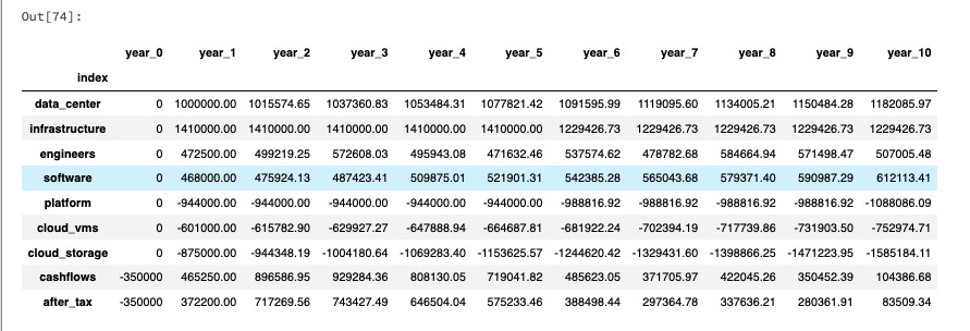
I picked this iteration to demonstrate that even though the NPV is always positive, we can see starting from year 2 our after_tax cash flows start to grind their way down. That is, there are a set of parameters that can start to work against us the longer we use cloud. This, by no means, implies this migration shouldn’t be considered. However, the business may want to examine longer time horizons as well as work with the vendors on guaranteed use discounts as well as other benefits. Additionally, we are missing out on some value-added benefits in this analysis so this isn’t the whole story but a warning to examine your data and results.
Next, let’s consider the two of the plots we generated, the 3 and 10 year NPV after tax.
| NPV 3 Years | NPV 10 Years |
|---|---|
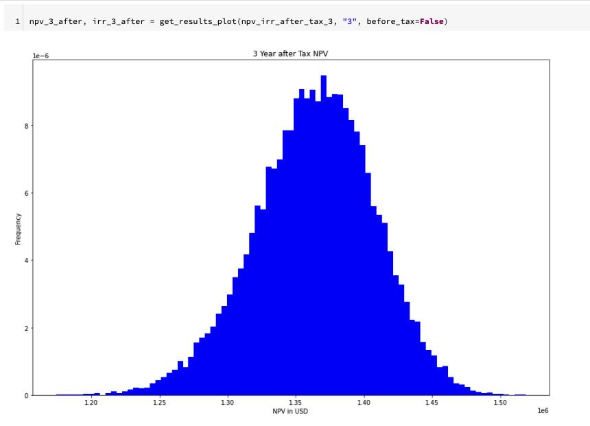
|
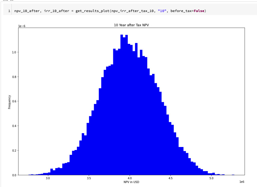
|
We can see with the following cash flows, our decision to move to cloud from on-premise would make sense, and provide value to our organization.
References
[1] Kenton, Will 2022, Capital Budgeting, Investopedia.com, accessed 11 March 2022, https://www.investopedia.com/terms/c/capitalbudgeting.asp
[2] Kenton, Will 2021, Monte Carlo Simulation, Investopedia.com, accessed 11 March 2022, https://www.investopedia.com/terms/m/montecarlosimulation.asp
[Capital Budgeting Notebook] Smith, Dustin 2022, Capital Budgeting Cloud Tutorial, accessed 11 March 2022, https://github.com/tdg-analytics-platform/capital-budgeting-python